0:01
Welcome to Excel Wiz. In today's video,
0:03
I'm going to show you how to highlight
0:05
the top three values in each row in
0:07
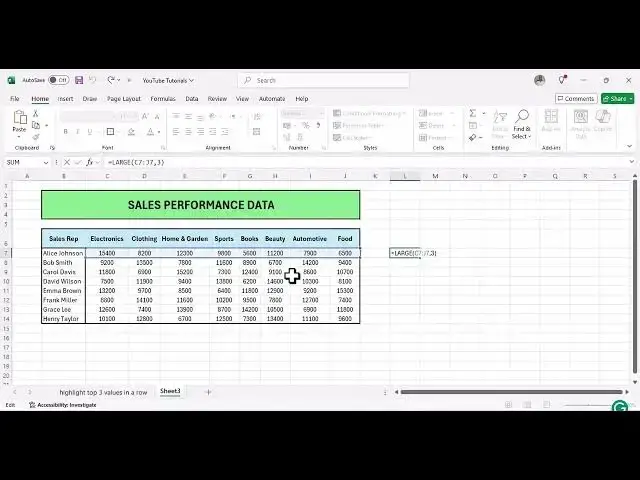
Excel. As you can see in this sales
0:10
performance data I have here. So I have
0:13
sales reps and they have each categories
0:17
um under which they have done the sales
0:20
and as you can see starting with Alis
0:22
Johnson the highest three values they
0:24
have is 15,400 12,300
0:30
and it goes all the way down to Henry
0:33
Taylor. But now assume now you're a
0:39
um a sales manager sorry and you have
0:42
this data here different from the first
0:44
one that you've just seen and you need
0:46
to pick out the three the top three
0:49
values it's very hard for you to tell
0:51
but when you have this it's easy for you
0:53
to just uh highlight and see the
0:56
numbers. So what I'm going to do I'm
0:58
going to try I'm going to show you how
1:00
you can achieve this in less than 5
1:02
minutes and please stay around and see
1:05
how this will be done. So let's get
1:11
So our sales performance data that we
1:14
have here. So the first thing we can
1:16
actually do uh normally you could just
1:19
um highlight the values. Let's do this.
1:21
Highlight the values. Click on
1:23
conditional formatting
1:26
uh top bottom rows and then you click on
1:29
top 10 uh top 10 items.
1:32
With top 10 items, it highlights the top
1:35
10 uh values for the whole range. But
1:38
now we need three. If you go all the way
1:42
down to three, it's going to highlight
1:44
the top three values, but now for the
1:46
whole range, which is not what you want.
1:48
We want top three values for each
1:51
particular row. So since this is not
1:54
what we want, let's clear this.
1:58
Let's clear this and then I'll show you
2:00
how now you can highlight the top three
2:02
for each uh row. So move to an empty
2:05
cell and we have to create a formula.
2:08
The formula is going we are going to use
2:11
the large uh function. So type in your
2:17
and then select the range of we start
2:20
with Alice Johnson. Select the whole
2:22
range from electronics all the way to
2:24
food. And then since we want to know the
2:28
that highest value, you write three and
2:30
then close your parentheses and hit
2:33
enter. So as you can see 11,200,
2:36
this is the that large value in this
2:40
particular row. This is not what we
2:43
need. So what we need is three values in
2:47
each in this row which are large. So
2:50
what we need to add something uh in this
2:54
So in this formula we are going to add
2:57
uh the first we are going to ask
3:02
uh the this first cell here is it
3:05
greater or equal to the third largest uh
3:10
the third largest value. So if that's
3:12
true then it's going to return true to
3:15
click enter. As you can see it says it's
3:18
true. So since uh we need this formula
3:22
but now since we going to drag it all
3:24
the way down it's going to change as we
3:26
drag it down. So what we can do we are
3:29
going to lock in our rows uh by
3:37
to lock the to lock the row. So once
3:40
that's done click enter. So move back to
3:44
this. What we are going to do now before
3:47
you go to conditional formatting ensure
3:50
you have your formula copied. So let's
3:54
copy the formula and then escape. Click
3:57
escape to get out of it and highlight
4:00
all the values once again. So once
4:02
that's done, go back to conditional
4:05
formatting. In this time, click on new
4:10
and then we are going to use to to
4:12
select use a formula to determine which
4:15
cells to format. Click on that and then
4:17
remember the formula we had. Paste it
4:20
here and then go click on format. So now
4:24
we can choose a color that is going to
4:27
to appear on fill. Uh let's say we go
4:31
with this green color. Click on this
4:34
green color and click on okay.
4:37
Click on okay. As you can see now for
4:40
every row we have 15,400 12,300
4:46
These are the top three values for Alis
4:48
Johnson. When you move down to Henley
4:53
we have 12,800, 12,500 and 3,400.
4:57
These are his top three values for each
5:02
for each category up here. So this is
5:06
how you can actually highlight top three
5:08
values in each row. You just have to
5:11
ensure that you have your correct
5:13
formula. I hope you have gained value
5:16
from this from this video and if you
5:19
have any questions please feel free to
5:21
ask in the comment section and if you
5:24
like this uh video please like subscribe
5:27
and see you again in the next video for