How to create floating cells in Excel

Floating cells in Excel allow you to keep specific data visible while you work on other parts of your worksheet. One effective way to achieve this is by using the Watch Window feature. This tool is particularly useful for monitoring important cells without constantly scrolling back and forth. Here’s a step-by-step guide on how to use the Watch Window or Snapshot feature to create floating cells in Excel.

Note that floating cells is different from freezing panes which makes rows and columns float.

Method: Using Watch Window

The Watch Window allows you to keep an eye on critical cells in your workbook while you navigate through other areas. This feature is ideal for tracking changes and monitoring data in real-time.

Steps to Create Floating Cells Using Watch Window:

1. Open Your Excel Workbook: Start by opening the Excel workbook you want to work on.

2. Select the Cells to Monitor: Identify the cells you want to keep track of. These could be important data points, totals, or any cells whose values you need to monitor constantly.

3. Access the Watch Window:

• Go to the Formulas tab on the Ribbon.
• In the Formula Auditing group, click on Watch Window.

4. Add a Watch:

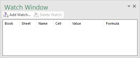
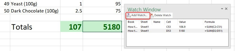
• The Watch Window will appear. Click on the Add Watch button.
• A dialog box will appear prompting you to select the cells you want to watch. You can manually enter the cell references or use your mouse to select the cells directly in your worksheet.
• After selecting the cells, click Add.

5. Monitor the Cells:

• The selected cells will now appear in the Watch Window. This window will display the workbook name, sheet name, cell reference, value, and formula (if applicable) of the watched cells.
• The Watch Window can be moved and resized to fit your workspace. You can keep it open while you work on other parts of your workbook, ensuring that you can always see the important data.

6. Using the Watch Window:

• As you scroll through your workbook, the Watch Window will remain visible, updating in real time to reflect any changes in the watched cells.

• You can add multiple watches if you need to monitor several cells simultaneously. Simply repeat the process of adding a watch for each additional cell or range of cells you want to track.

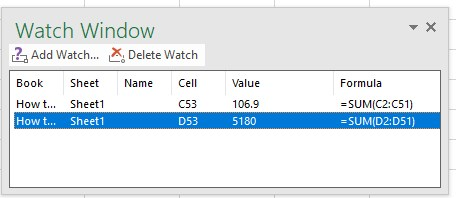
7. Removing a Watch:

• If you no longer need to monitor a specific cell, you can remove it from the Watch Window.
• In the Watch Window, select the cell reference you want to remove.
• Click on the Delete Watch button.

Download the practice template

Download

Method 2: Using the Camera Tool

The Camera Tool in Excel allows you to create a live snapshot of a cell range. This snapshot can float and remain visible as you scroll through your worksheet.

Steps to Use the Camera Tool:

1. Enable the Camera Tool:

• Go to the File tab and select Options.
• In the Excel Options dialog box, select Customize Ribbon or Quick Access Toolbar.
• From the list of commands, choose All Commands and find the Camera tool.
• Add the Camera tool to your Quick Access Toolbar or a custom group in the Ribbon.

2. Select the Range:

• Highlight the range of cells you want to create a floating snapshot of.

3. Create the Snapshot:

• Click on the Camera tool icon in your Quick Access Toolbar or Ribbon.
• Click on the location in your worksheet where you want the floating snapshot to appear. A picture of the selected range will be created.

• Position the Snapshot: You can move and resize the snapshot as needed. The snapshot remains live, updating automatically as the data in the original range changes.