
Conditional formatting based on another cell can help you create an interactive spreadsheet. For example, you can customize it to highlight all the sales in a data range that exceed your target file. Also, you can set a class mean score to a cell and use conditional formatting to highlight all students that scored below it.
The use cases for conditional formatting are endless, whether for business, school, work, etc. In this tutorial, I will highlight values based on another cell.
How to highlight values based on another cell
You need to apply formulas to highlight values based on another cell in Excell. The formula will determine if it meets the specified condition, then highlight it with your preferred colors. Here are some of the most used conditions for conditional formatting.
| Condition | Formula Example |
| Greater Than | =$C3>20 |
| Less Than | =$C3<20 |
| Not Equal To | =$C3<>20 |
| Equal To | =$C3=20 |
| Greater Than or Equal To | =$C3>=20 |
| Less Than or Equal To | =$C3<=20 |
| Between | =AND ($C3>10, $C3<10) |
Download the practice workbook to follow along
Conditional formatting based on another cell less than
I have a list of students, marks, ages, and index numbers. For this example, I want to highlight students with less than 50 marks. However, I don’t want to highlight only the cells containing marks. The goal is to highlight the student alongside marks, age, and index number. This is a perfect example of how to conditional format based on another cell.

1. Highlight the range that you wish to apply conditional formatting to
2. Click on the conditional formatting drop-down menu and click on new rule

3. A new pop-up window will launch Once you click on a new rule. Under this section, select the last option, which says, “Use a formula to determine which cells to format”
4. Type the following formula under edit the rule description
=$G5<50
5. Click on the format button. Choose your preferred color and press ok

6. You’re ready to go Once you type the formula, select the color. Click on ok.

7. All the cells in your data will be formatted according to your formula

Conditional formatting based on another cell greater than
You need to use the greater than sign to highlight cells based on another cell greater than. The greater than sign is the opposite of the less than sign. Here is how to do it.
1. Select the range that you wish to apply conditional formatting to
2. Click on the conditional formatting drop-down menu and click on New rule

3. A new pop-up window will launch Once you click on a new rule. Under this section, select the last option, “Use a formula to determine which cells to format.”
4. Type the following formula under edit the rule description
=$G5>50
This formula will highlight all students that scored a

5. Click on the format button. Choose your preferred color and press ok
6. You’re ready to go Once you type the formula and select the color. Click on ok.
7. All the cells in your data will be formatted according to your formula

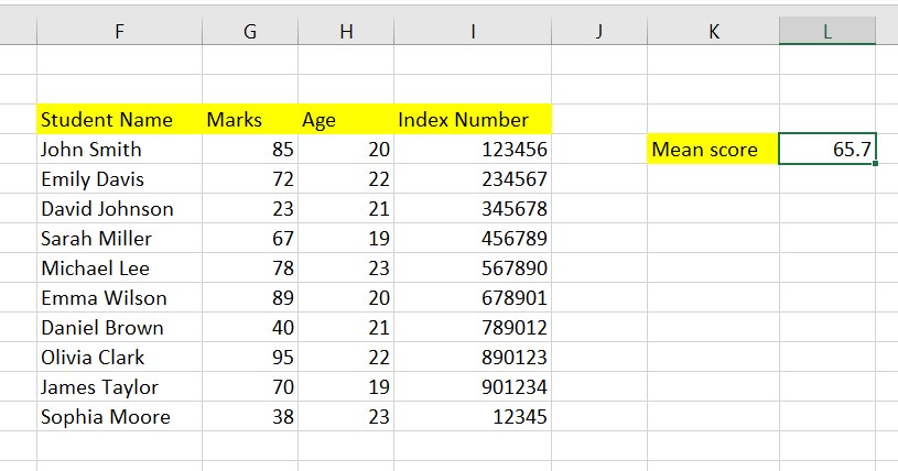
How to format a column based on a cell
Sometimes, you just want to color cells of a column based on a single cell. For example, in the data below, I have a column containing students’ marks. Cell L4 holds the mean score marks of the whole class. The task is to highlight only marks that are below the mean score.
1. The first step is highlighting the column you wish to format. (note that in this case, you need to highlight one column)
2. Now click on conditional formatting and click on new rule (A pop-up window will appear)
3. Under this window, click on “Use a formula to determine which cells to format.”
4. Type the following formula under edit the rule description
=$G4 < $L$4

5. Click on the format to choose and click on the fill tab to choose the color for highlighting.
6. Click okay, and the cells with less than the mean score reference in a cell will be highlighted.

Similar Reads:
How to Highlight Past Dates in Excel
How to count Blank cells in Excel
Discover more from Excel Wizard
Subscribe to get the latest posts sent to your email.